Code Snippets

This page is slowly getting outdated. I mostly use it to display videos. Please refer to:

Geophysics & Glaciology at Univ. Tübingen

for more up-to date information.

Traveltime inversion of wide angle data using raytracing and traveltime inversion

This is a code example using  a wide-angle radar dataset to constrain the radio-wave propagation speed, and with it the depth-density profile:

Constraining variable density of ice shelves using wide-angle radar measurements radar
R. Drews, J. Brown, K. Matsuoka, E. Witrant, M. Philippe, B. Hubbard, F. Pattyn; The Cryosphere

Traveltime Inversion using Raytracing and a continuous depth-density function

The raytracing forward model is based on:

Margrave, G. F.: Numerical Methods of Exploration Seismology with algorithms in Matlab, CREWES Toolbox Version: 1006 and requires the following files in a local folder “raytracing”:

You have to download these files and place them in a local folder “raytracing/”
drawray.m flipy.m shootray.m sphdiv.m surround.m traceray_pp.m

The code can be found here: http://www.codeforge.com/article/174599

 

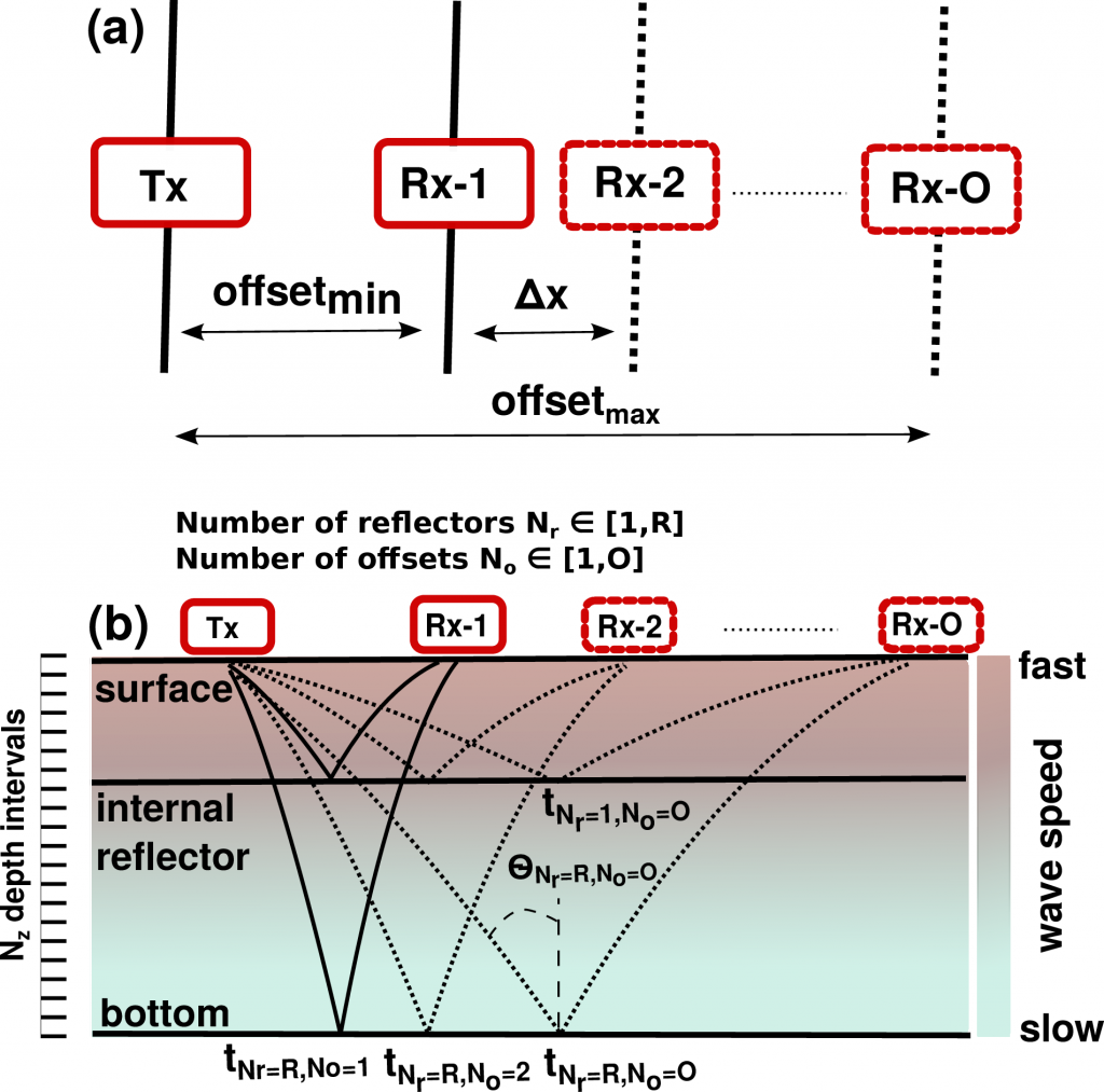
(a) Plain view of a possible wide-angle acquisition geometry: Transmitting (Tx) and receiving (Rx) antennas are aligned in parallel. While the transmitter remains at a fixed location, the receiver is incrementally moved farther away. A sketch of the corresponding raypaths is shown in (b) with a synthetic velocity-depth function color coded.

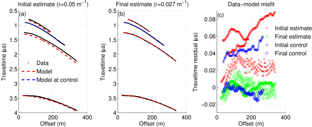
Example for initial (a) and final (b) fit between the raytracing forward model and the reflectors for real data collected in Antarctica. In this case, three reflectors (black dots) were used for the inversion and one reflector was kept for control. The forward model corresponds to the red dashed curves and the control relectors to the blue dashed curves. Initial estimates shown here were r = 0.05 1/m , D 1 = 68.2 m, D 3 = 112.9 m, D 4 = 291.2 m; the best fit resulted in r = 0.027 1/m , D 1 = 67.7 m, D 3 = 111.2 m, and D 4 = 293.3 m. The traveltime residual between model and data for initial (x) and final fit (o) are shown in (c).